This blog series is a set of notes that expand on Dr Shirley’s “Ray Tracing The Rest of Your Life” book. The book is compact, introducing all the tools that one will need in their arsenal to build a sophisticated ray tracer. I found it very refreshing in terms of simplifying otherwise esoteric concepts and bridging the gap between simple mathematical concepts and their application in ray tracing.
My journey through the book raised many questions, which Dr Shirley was very helpful in answering and explaining. Along the way I read many different articles and saw different videos to understand things. I am probably not the only person who needed help understanding things and won’t be the last, so I thought it would be a good idea to share the information that I gathered.
The format of this post is unconventional - you should have a copy of the book (ideally the PDF as it is the most recent updated) open in another tab. I’ll try to guide you as best as I can throughout the book by asking you to look at the book and come back when you reach a certain point.
These statements will be in bold and red!
Re-reading is also very important - it’s very hard to understand everything at a first read. Don’t worry too much if you don’t get everything immediately. These are not straightforward concepts so just keep at it. If you feel truly stuck, reach out to me and we’ll try to clear things up. With all that said, let’s start.
Chapter 1: A Simple Monte Carlo Program
The first chapter is very straightforward. Demonstrating Monte Carlo by estimating \(\pi\) is a prevalent computational statistics example.
The code snippet for this that is presented in the book is very simple and self explanatory. A point is generated inside a square and if it is inside the circle, we increase the counter tracking the number of points inside the circle. We divide this final count by the total number of points we generate to get an average answer to \(\pi\).
It’s time to go look at the book - read up until the you get to the 2nd code snippet, involving the running \(\pi\) calculation program.
One of the questions of those uninitiated in probability and Monte Carlo theory might be: How does this type of computation work and how does it end up giving us an estimate of \(\pi\)? This stems from what is known as the expected value.
A classic example in explaining the expected value is trying to answer the question:
What is the probability that I will get a heads, when I flip a fair coin?
We know intuitively that it is 0.5. However what the expected value theory shows us is that if we
- get an actual fair coin,
- start flipping it,
- take note of each result,
- count the number of heads and tails,
- average them,
We will probably get a result close to 0.5. The more times we toss the coin, the closer to 0.5 the answer will be.
The mathematical notation used to describe the expected value is:
\[E[X] = \sum_{i=1}^k x_i p_i = x_1 p_1 + x_2 p_2 + ... + x_k p_k\]
- \(E[X]\) is the expected value of \(X\), our statistical experiment.
- \(x_i\) is the result of each sample that we compute of our function
- \(p_i\) is the probability weight of this sample. They must sum up to 1.
I’ll use another example rather than a coin toss to tie with the above equation. If we had a fair 6-sided dice, the expected value would be:
\[E[X] = \sum_{i=1}^k x_i p_i = \frac{1}{6} + \frac{2}{6} + \frac{3}{6} + \frac{4}{6} + \frac{5}{6} + \frac{6}{6} = 3.5\]
where \(x_i\) was the dice roll and $$ \frac{1}{6} was the probability weight. If dice wasn’t fair, the weights would be different - that doesn’t matter as long as they sum up to one.
Back to our original monte carlo example, the reason why this works is a theorem known as the Law of Large Numbers. The weak law of large numbers states that if we take a number of samples and average them, it will PROBABLY converge to the expected value. The strong law of large numbers states that it will converge ALMOST SURELY (with probability 1). We’re not going to go down this rabbit hole, the one of interest to us in the weak law.
An important term that we should define is variance. In our example, we were trying to compute \(\pi\), which makes this the mean we’re trying to estimate. The variance, in very informal language, measures how spread out our sample computations are from this mean. The lower the variance, the less spread out the samples are and the more accurate our computed mean is to the expected value (the expected value is also known as the mean). If we have high variance, this means our samples are spread out, and we might be using an ineffective function to computationally find our mean. There are ways to quantify variance which are useful for estimating the error of our Monte Carlo techniques, however I think it would not be fruitful for now to discuss those.
The Law of Diminishing Returns explains the idea that the more samples we take, the more we need than before, to get an accurate answer. In terms of numbers, if you want to half the error that you’re getting, you’ll need to quadruple the amount of samples. Here is how the error between our estimated value of \(\pi\) and actual \(\pi\) decreases as we compute more samples.
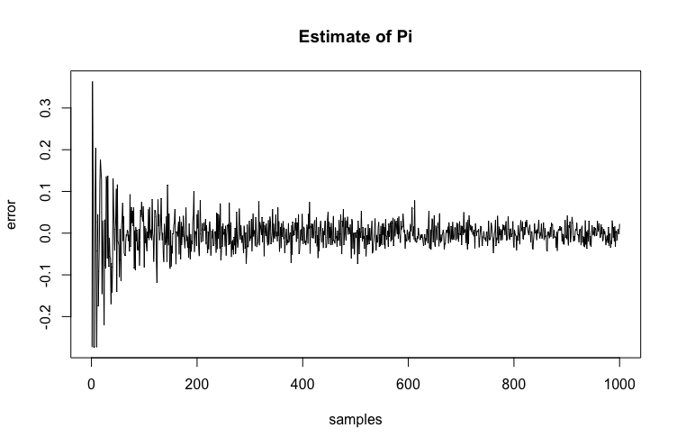
Notice how after sample 200, the error doesn’t decrease that much. This doesn’t hold a lot of significance for now but it’s good to keep this in mind.
Now would be a good time to go read the rest of the chapter.
Stratification is a way of intelligently placing your samples to estimate your function better. If you look at my blog post about random numbers, I show that a good PRNG (Pseudo-Random Number Generator) should generate uniformly distributed points. When you’re dealing with multiple dimensions a PRNG’s inherent randomness isn’t enough. Think of dimensions this way: you need 2 uniform random numbers for your primary ray, then 2 for your lens, then another 2 for your next bounce and so forth. Everytime, you’re adding another dimension and although your random numbers are unifornm if we look at them at being in the same dimension, it may not necessarily be the case when used in these different dimensions. To ensure true uniformity, without having clustered samples, we stratify the samples we take.
The careful selection of samples to minimize variance is an ongoing area of research, that is an absolutely fascinating subject and one of my favourite topics in CG. Dr. Shirley expands on this topic is in this blog post: Flavors of sampling in ray tracing. Leonhard Grünschloß has some excellent implementations of different Quasi-Monte Carlo based samplers.
I’ll slightly re-visit stratification at the end of Chapter 2, once we define the Monte Carlo Integral and importance sampling. The topic warrants tons of blog posts, maybe someday…
The next post will focus on Chapter 2, where I’ll delve ever so slightly into Monte Carlo theory and we’ll perform some interesting computations.
If you have any questions and feedback, feel free to comment or contact me via twitter/email.
comments powered by