In this post I’ll talk a bit about pseudo random number generation. This will be the first in an assortment of posts regarding monte carlo methods.

I’ll assume you have working knowledge of calculus and some probability and statistics.

The most essential aspect of any form of monte carlo method is the generation of random numbers. Uniformly distributed random numbers on the interval [0,1] are what we’d like to generate first, as they are also what is required for the other types of distributions.

Generating random numbers using a pseudo random number generator (PRNG) means that we generate a sequence of numbers, using some particular seed value (some arbitrary constant) that initializes the random number generation algorithm. We use the term pseudo, because the numbers generated are not truly random but generated deterministically and hence can be replicated if the same seed and the same constants in the function are used. This is ideal for us, so that we can replicate and debug our algorithms. We can think of these algorithms as generating a deterministic sequence which is based on a starting point.

For this sequence to be considered to be of good quality, it should have certain properties, such as lack of predictibility (i.e. if we generate x values, and we can guess the next, this means the predctibility is possible) and equidistribution. For example if the mean of a large sequence of uniformly distributed numbers in the range [0,1] is not 0.5, then it is likely that something is wrong with the PRNG, given that due to the Law of Large Numbers, we would expect the arithmetic mean of this sequence to be similar to the expected mean (the expected mean being 0.5). We won’t focus on hardcore evaluation PRNGs and leave that to other minds, some useful links are “How random is pseudorandom testing pseudorandom number generators and measuring randomness” and TestU01 tests. We’ll look at 2 PRNGs and do some simple tests to measure their quality.

Let’s look at a simple PRNG known as the Linear Congruential Generator (which I’ll now continue referring to as LCG).

The LCG is an easy-to-implement PRNG, the function definition being:

where:

• m is the modulus constant, and m > 0.
• a is the multiplier, and 0 < a < m.
• c is the increment, 0 <= c <= m.
• X₀ is the seed value, 0 <= X₀ < m.

The above constants are all integers. Careful selection of these values ensures that the sequence we get is of a high quality.

Here’s an R listing of what the code for this should look like:

lcgen <- function(x0=4, N, a=1229, c=1, m=2048)
{
  x = c()
  x[1] = x0
  for(n in 2:(N+1))
  {
    x[n] = (a * x[n-1] + c) %% m
  }
  return (x[2:(N+1)]/m)
}

N is the number of random numbers we want to generate. Let’s generate 1000 samples and plot a histogram to look at the distribution.

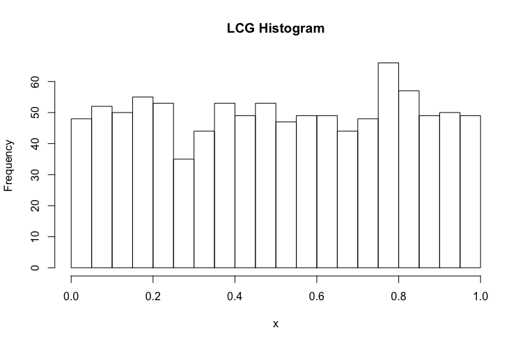
It’s fair to say, the distribution of samples looks good. Given that the generation of a value is dependent on the next let’s see if we can see a pattern by plotting them in a time series.

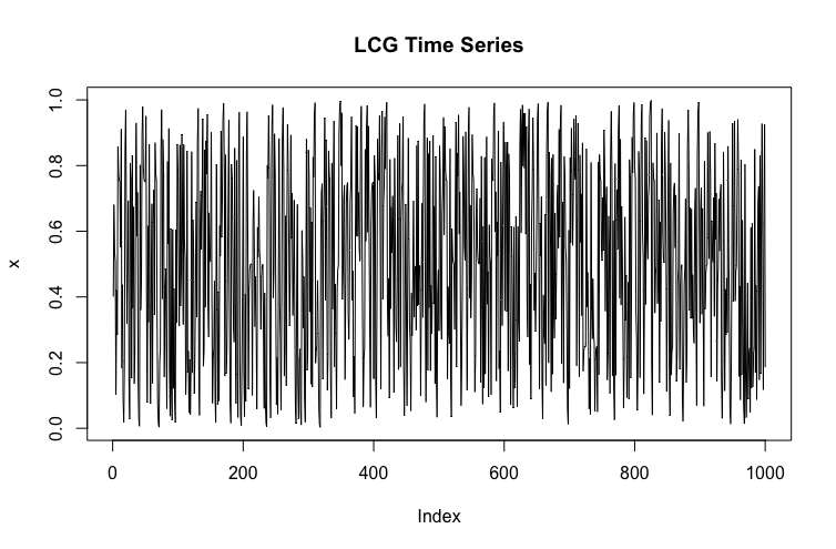
That looks pretty random, so let’s plot them in series, taking pairs as cartesian coordinates (x_2k-1, x_2k). This type of test is known as autocorrelation.

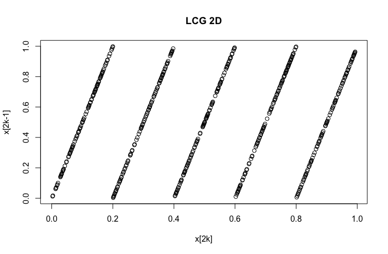
Well that’s interesting, pairs line up as lines… what if we plot them in 3D?

The numbers are forming a line in 2D, a plane in 3D and this pattern continues in n-dimensions, where a n-dimensional hyperplane is formed for the n’th dimension. George Marsaglia identified this issue in 1968 and it is now know as the Marsaglia Theorem. He pointed out the worrying conclusion that all the papers that had used a LCG as their PRNG of choice might have wrong results. This highlights the importance of using a good PRNG.

From now on we’ll use a PRNG of a higher quality, the Mersenne Twister. I won’t go into its implementation, it’s a lot more sophisticated and robust than the LCG. The more recent PCG PRNG is better than Mersenne and it’s what I use in my rendering system. Having said that, R’s runif (short for random uniform) command uses the Mersenne Twister algorithm, and for these posts it should suffice. PBRT 2 used to use Mersenne Twister and PBRT V3 uses PCG.

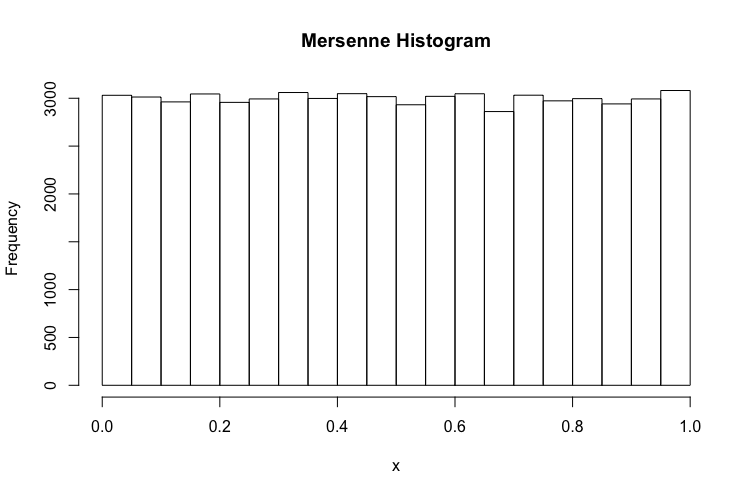
If we re-run the above tests using Mersenne Twister, we can see that, the histogram looks acceptable,

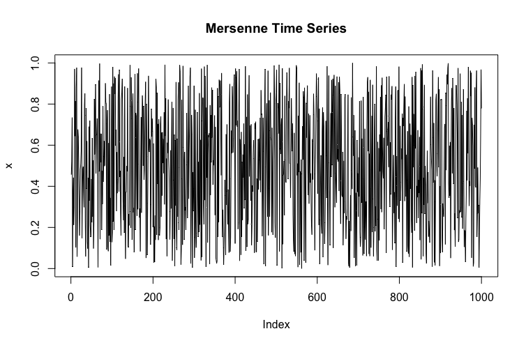
so does the time series plot,

and the 2D plot (points look to be well distributed in the 2D plane)

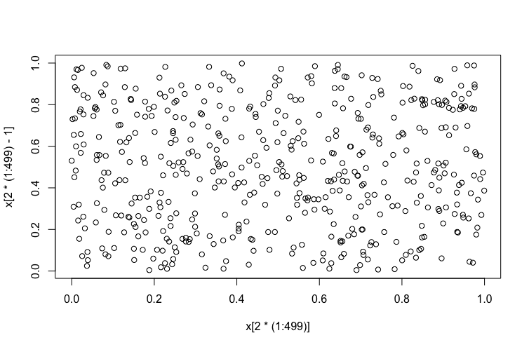
and the 3D plot (points look to be well distributed in the 3D unit cube).

Whenever you see runif, assume the numbers are well uniformly-distributed using the Mersenne Twister algorithm. Now that we’ve understood a bit more how uniform random numbers are generated, I’ll later post about transforming these uniform random numbers into other forms of distributions, e.g. normally distributed.