Welcome back! If you’re joining from the 1st post, you can skip ahead and start reading from the Chapter 2 title. If not, here’s a link to the first post as there’s some information in the beginning about this blog series.
Chapter 2: One Dimensional MC Integration
Monte Carlo is widely used to solve integrals of higher dimensions, where an analytical method is not possible, or other integral computational methods are intractable. Dr. Shirley selects a simple integral to show how effective Monte Carlo integration is.
Start reading the chapter right until you get to the code that computes the integral. Don’t worry if you don’t get it, I’m going to explain everything.
The integral is \(\int_0^2 x^2 dx\) which will compute the area under the curve, with the limits 0 to 2. So how do we translate this into a Monte Carlo estimate? I was a bit confused by the sudden appearance of the 2 being multiplied with the average(x^2, 0, 2) function. Why are we multiplying the sample average by 2? Well as it turns out, this how we perform Monte Carlo integration. A generic integral of the form:
\[F = \int_a^b f(x)\]
can be estimated with a Monte Carlo estimator by performing
\[(b-a) \frac{1}{N} \sum_{i=0}^{N-1} f(X_i)\]
\(x_i\) are uniformly distributed random numbers between 0 and 1, and \(N\) is the number of samples you pick.
Read the book right up until he proposes making his own PDF. I’ll lengthen the explanation and drive in a bit of probability, enough to show you the ropes but not enough to bore you (hopefully).
So the area function Dr. Shirley is trying to calculate is:
\[\int_0^2 C' r dr = \frac{1}{2} [C'r^2]_0^2 = 2C'
\\
1 = 2C'
\\
C' = \frac{1}{2}\]
Knowing that \(p(r) = C'r\) this leads to \(p(r) = \frac{r}{2}\). The rest is pretty readable and understandable so I’ll move onto something else.
A short introduction into probability theory with a bit more formality will go a long way into helping you understand what Dr. Shirley computes in the book and other future graphics problems.
We’ve been talking about random variables for a while. We know that generating a uniform random variable means that we use a function to generate a number in a particular range and since we stipulated that it is uniform, this also means that any other number in that range could have been picked with the exact same probability.
We’ll introduce some terms.
- \(X\) represents the random variable. Since we’re using random variables to estimate something, this also is referred to as a random variable!
- \(P(X)\) represents the probability of \(X\).
- \(P(X = x)\) represents the probability that \(X\) is a particular value \(x\).
To exemplify these terms, in our statistical experiment we are going to toss a coin twice.
- \(X\) is the number of heads that we get. This is the random variable that is the result of our 2 coin tosses. \(X\) will either be 0 (\(TT\)), 1(\(HT\) or \(TH\)) or 2(\(HH\)).
- \(P(X)\) will be the probability of getting 0, 1 or 2 heads.
- \(P(X = x)\) will be a particular sequence of coin tosses, such as \(TT\) or \(TH\).
The cumulative distribution function (CDF) and the probability mass/density function (pmf/PDF) are the 2 pillars of understanding the nature of a random variable. The reason I used mass/density is because mass is used when we are describing a discrete distribution, and density is used in the continuous case. In this example, it’s the pmf (a coin toss is a discrete experiment) that I’ll be talking about, however the same ideas hold for the PDF.
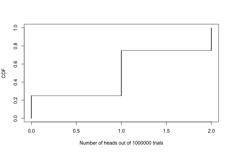
This is the CDF of the experiment above:
| \(P(X)\) |
CDF \(P(X <=x)\) |
| 0 |
0.25 |
| 1 |
0.75 |
| 2 |
1 |
As you may have noticed, the CDF is maxed out at one. 1 is the upper limit of the probability that an event from an experiment occurs - 0 is the lower limit. It is called cumulative because the probability distribution accumulates with each event. If you haven’t understood what that table is representing, let’s use our words!
- \(P(X=0)\) means that that probability of getting no heads is 0.25.
- \(P(X<=1)\) is \(\)P(X=1) + P(X=0)\(\). \(P(X=1)\) is \(TH\) and \(HT\) and therefore we’re adding 0.5 to the probability of getting \(TT\) which is 0.25, hence 0.75.
- \(P(X<=2)\) is just the probability of \(HH\) (0.25) + the previous 0.75, our final result being 1.
This is what the CDF looks like when we plot it
So can you guess what the PMF will look like? Hint: the pmf will describe the probability of each occurring coin toss .
| \(P(X)\) |
PMF \(P(X =x)\) |
| 0 heads |
0.25 |
| 1 heads |
0.5 |
| 2 heads |
0.25 |
If you sum up all the probabilities, they’ll add up to 1. So the PMF is showing us the probability of an event occurrence and CDF is showing us the probability of a range of events occuring. I know I keep on repeating this statement, but it’s common to not fully grasp the difference between the CDF and PMF and be unsure of their purpose. If you look hard at both, see you can go from the CDF to the PMF and vice versa.
So what happens if we’re dealing with continuous cases?
Well for starters, the PMF changes to a PDF. We are also usually presented with functions to represent the CDF and PDF. To find the CDF from the PDF, we integrate the PDF from \(-\infty\) to \(x\), where \(x\) is a placeholder variable.
I’m not going to show an example because at this point I think you should go back to the book but wait until this final concept.
We’ve mentioned that we have been generating uniform random variables using a PRNG. In many cases however, we would like to take these uniform random numbers and would like to make them follow some other kind of distribution. We want to transform them. The way to go about this is a technique known as the Inverse Transform method. The technique is very simple and very powerful:
Let’s say we have a random variable \(X\) , that has a CDF \(F(X)\). We want to generate values distributed according to this distribution. The steps to do this are:
- Generate a uniform random number u between \([0,1]\).
- Find the inverse of the CDF of \(F(X)\).
- We find X by computing \(F^{-1}(u)\). \(X\) is now distributed according to \(F(X)\).
The Inverse Transform method warrants its own blog post so I won’t go into detail about its intrinsics and its edge cases and so forth.
Go back to the book and come back right after you’ve obtained the inverse of the CDF.
We have computed a Monte Carlo estimation of an integral, and now we’ve computed the inverse cdf of a PDF, which means we can transform our uniform random numbers into the PDF that we selected. If you recall, we said that we draw our samples from a uniform distribution from 1 to 0 in our original definition of the Monte Carlo estimator. The PDF of this estimator is \(\frac{1}{1-0}\) which is \(1\). The more general Monte Carlo estimator definition is actually this:
\[\frac{1}{N} \sum_{i=0}^{N-1} \frac{f(X_i)}{p(X_i)}\]
Where \(p(X_i)\) is the PDF from which the samples are drawn. By selecting a PDF that matches the shape of the function that we are trying to estimate, we are weighting the samples so as to reduce the variance. This is known as Importance Sampling! Choosing a good PDF is an ongoing form of research. For our integral, the PDF Dr Shirley’s picked is \(\frac{1}{r}\).
For the moment, we’ve been drawing samples from the uniform distribution, but thanks to the inverse transform method, we’re now using these uniform numbers and transforming them to match the new PDF. We’ll then compute our original integral with these new random variables and divide by the new PDF.
Now would be a good time to finish the chapter.
If you feel more mathematically inclined, Alan Wolfe has a great blog post about One-Dimensional Monte Carlo Integration. He’s also got a plethora of posts that will have some common content with this blog post series. I would also suggest you have a look at PBRT Chapter 13 if you’re feeling brave!
If you remember, we spoke about stratification previously. Let’s take the original integral \(\int_0^2 x^2\). To stratify the points, we’ll divide the interval in 4 bins. If I am taking N samples, we are going to take \(\frac{n}{4}\) samples per bin, so let’s call this value \(k\). The Monte Carlo estimate using stratified sampling now looks like this:
\[\int_0^2 x^2 = (0.5 - 0)\frac{1}{k} \sum_{i=0}^{k} x_1^2 +
(1.0 - 0.5)\frac{1}{k} \sum_{i=0}^{k} x_2^2 +
\\
(1.5 - 1)\frac{1}{k} \sum_{i=0}^{k} x_3^2 +
(2 - 1.5)\frac{1}{k} \sum_{i=0}^{k} x_4^2\]
\(x_1\) is a random number between 0 and 0.5, \(x_2\) is between 0.5 and 1.0, \(x_3\) between 1.0 and 1.5, and \(x_4\) between 1.5 and 2, giving us a total of \(N\) samples.
Here is a self contained program showing the stratified and naive Monte Carlo estimations.
#include <iostream>

int main()
{
	float simpleMcRes = 0.0;
	int samples = 1000000;
	float res = 0.0f;

	int bins = 10;
	int samplesPerBin = samples / bins;

	for(int i = 1; i <= bins; ++i)
	{
		float binStart = (i - 1.0f) / float(bins);

		std::cout << binStart << std::endl;
		for(int j = 0; j < samplesPerBin; ++j)
		{
			float x = 2 * drand48();
			simpleMcRes += x * x;

			x = 2 * (i + drand48() - 1.0f)/float(bins);
			res += x * x;
		}
	}

	simpleMcRes = 2.0 * simpleMcRes / float(samples);
	res = 2.0f * res / float(samples);

	std::cout << "Simple MC: " << simpleMcRes << std::endl;
	std::cout << "Stratified MC: " << res << std::endl;

	return 0;
}
Stratification warrants its own post following some discussions with some friends. I wanted to show certain properties but felt that this post would be too long.
That’s pretty much it for this post, next up is Chapter 3 and 4.
If you have any questions and feedback, feel free to comment or contact me via twitter/email.
comments powered by